Named ranges in Google Sheets

A named range is a feature in Google Sheets that lets you give a range a range a unique name. This is a very useful feature since you can use the name of range in formulas and functions instead of using its A1 notation.

For example, if you have a spreadsheet that you use for budgeting, you might have two named ranges called Expenses and Income. You can then reference these ranges in formulas and functions by using their name. So instead of =SUM(Sheet2!A3:A17), you can use =SUM(Income). Using names for ranges instead of their A1 notation makes formulas and Apps Script code easier to understand.

Prerequisites

This tutorial will assume that you are familiar with:

• The concept of a range in Google Sheets.

• How to read data from and write data to a range in Google Sheets using Google Apps Script.

• The basics of coding in Google Apps Script.

Why should you use named ranges in Google Sheets?

There are several benefits to giving meaningful names to ranges in your spreadsheet.

• Make your formulas and scripts easy to read and understand

• Giving variables a meaningful descriptive name is a best practice in coding. Doing so helps others read and understand your code.

• Similarly, you can think of a range in a spreadsheet as a variable that references an array of data. Therefore, it is a best practice to name ranges that get used in multiple places in your spreadsheet.

• You only need to edit range references in one place

• If you need to make changes to a range that is used in multiple formulas and scripts, you only need to make this change in one place if you're using a named range.

• All of the formulas and scripts will immediately use the edited range. This prevents errors that result from formulas using an outdated range reference.

How to create a named range in Google Sheets?

There are two ways to create a named range: (1) manually using the Google Sheets UI and (2) using Apps Script code.

Creating a named range using the Google Sheets UI

There are two ways to create a named range using the Google Sheets UI:

1. Select a range, right click and select Define named range. Then enter a name for this range and select Done.

2. Select Data —> Named ranges from the menu. Then create the named range from the sidebar by entering a name and selecting the range.

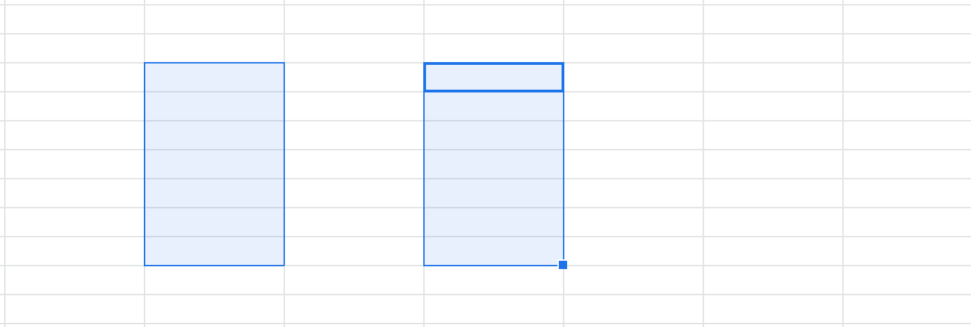
Note: You cannot name a list of ranges

In the screenshot below, two ranges have been selected. Google Sheets currently does not support assigning a single name to a list of ranges.

Note

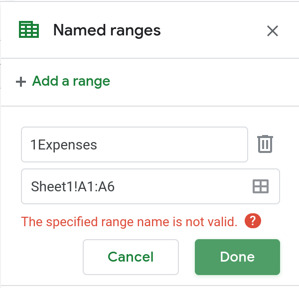
According to Google's documentation, the following restrictions apply to names of ranges.

• They can contain only letters, numbers, and underscores.

• They can't start with a number, or the words "true" or "false."

• They can't contain any spaces or punctuation.

• They must be 1–250 characters.

• They can't be in either A1 or R1C1 syntax. For example, you might get an error if you give your range a name like "A1:B2" or "R1C1:R2C2."

When you enter a name that is not valid, the UI will warn you.

Creating a named range using Google Apps Script

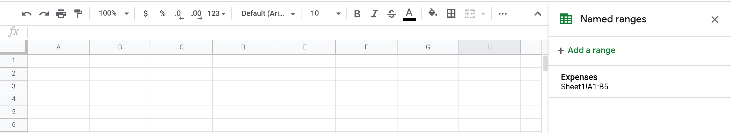
To create a named range using Apps Script, use the setNamedRange() method of the Spreadsheet object. The method takes two arguments as input: (1) the name of the range (2) the range itself.

function createNamedRange() {
  var ss = SpreadsheetApp.getActive();
  var range = ss.getRange("Sheet1!A1:B5");
  ss.setNamedRange("Expenses", range);
}

Running the above function will create a named range called "Expenses" that is a reference to the range Sheet1!A1:B5.

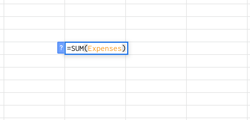
How to use a named range in a Google Sheets formula?

Using a named range in a formula is straightforward. Just use the name instead of specifying the range's A1 notation. For example, instead of =SUM(Sheet1!A1:B5), use =SUM(Expenses) instead.

Working with named ranges in Google Sheets using Google Apps Script

Reading data from a named range using Apps Script

To read data from a named range, first reference the named range by using the getRangeByName() method of the Spreadsheet object. Then, read the values in the range by using the getValues() method.

function readNamedRange() {
  var range = SpreadsheetApp.getActive().getRangeByName("StudentGrades");
 var values = range.getValues();
 Logger.log(JSON.stringify(values));
}

Writing data to a named range using Apps Script

To write data to a named range, first reference the named range by using the getRangeByName() method of the Spreadsheet object. Then, write a two-dimensional array of values to the range by using the getValues() method. Note: the size of the array (i.e., the number of its rows and columns) must be the same as that of the named range.

The code below writes the two-dimensional array dataToBeWritten into the range named StudentGrades.

function writeToANamedRange() {
  var range = SpreadsheetApp.getActive().getRangeByName("StudentGrades");

  var dataToBeWritten = [
      ["Student", "English Grade", "Math Grade"],
      ["Erik B", "A", "C"],
      ["Lisa K", "B", "A"],
      ["Faye N", "A-", "A"],
      ["Rose A", "B", "B"],
      ["Derek P", "B-", "A-"]
  ];

 range.setValues(dataToBeWritten);
}

Using named ranges with custom functions in Google Sheets

You can use named ranges as arguments when calling a custom function from a cell in your spreadsheet. However, when you do this, the function will never know that it was passed a named range. Instead, it will directly receive the data that is contained in the named range that was passed to it as an argument.

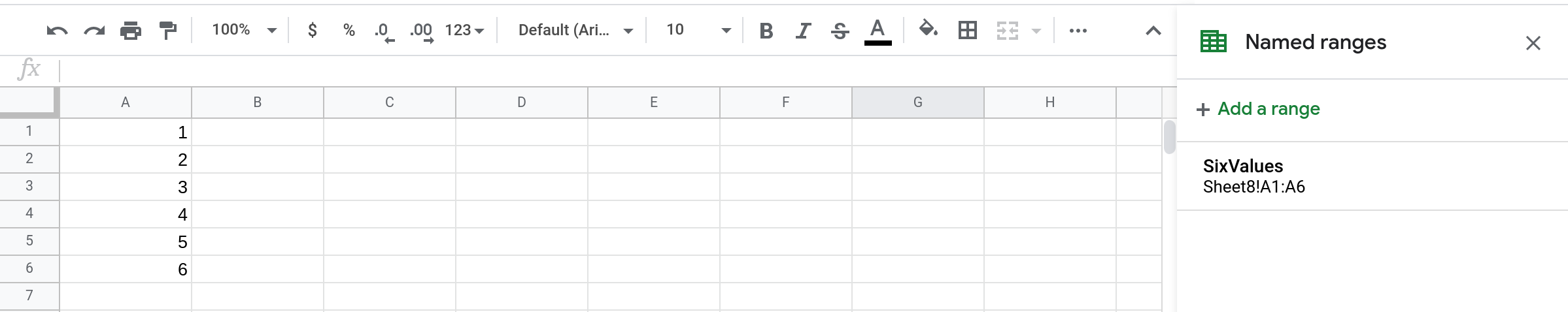
Let us say the range Sheet8!A1:A6 contains 6 number values: 1, 2, 3, 4, 5 and 6. This range has the name SixValues.

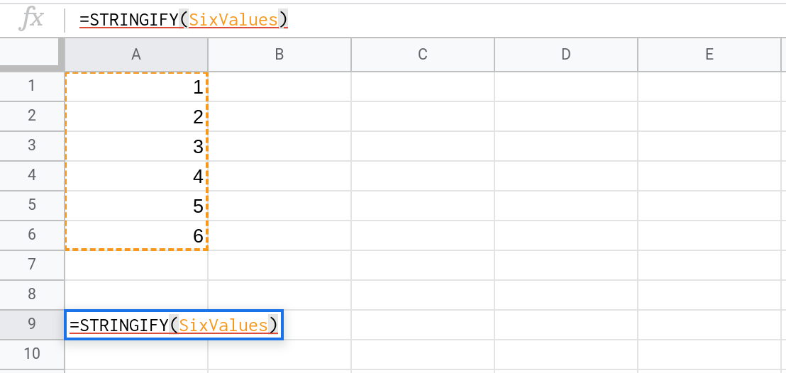
Now, let's write a custom function called STRINGIFY() that returns the JSON string representation of the argument that is passed to it.

function STRINGIFY(value) {
  return JSON.stringify(value);
}

When you call the function STRINGIFY() with the named range SixValues as the argument, you'll see that the value returned is the string representation of the two-dimensional array of values contained in the range Sheet8!A1:A6. The function STRINGIFY does not know that you called it with a named range or even a range. It only sees the values in the range that you passed as an argument to it.

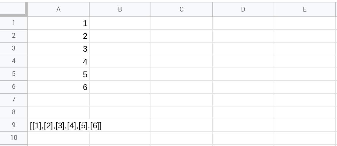
The value [[1],[2],[3],[4],[5],[6]] is the JSON string representation of the two-dimensional array below. The outer array contains rows and each inner array contains the values in each row (i.e., its columns).

[
  [1],
  [2],
  [3],
  [4],
  [5],
  [6]
]

Reading all the named ranges in a Google Sheets spreadsheet

To read all the named ranges that have been defined in your spreadsheet, use the getNamedRanges() method of the Spreadsheet object.

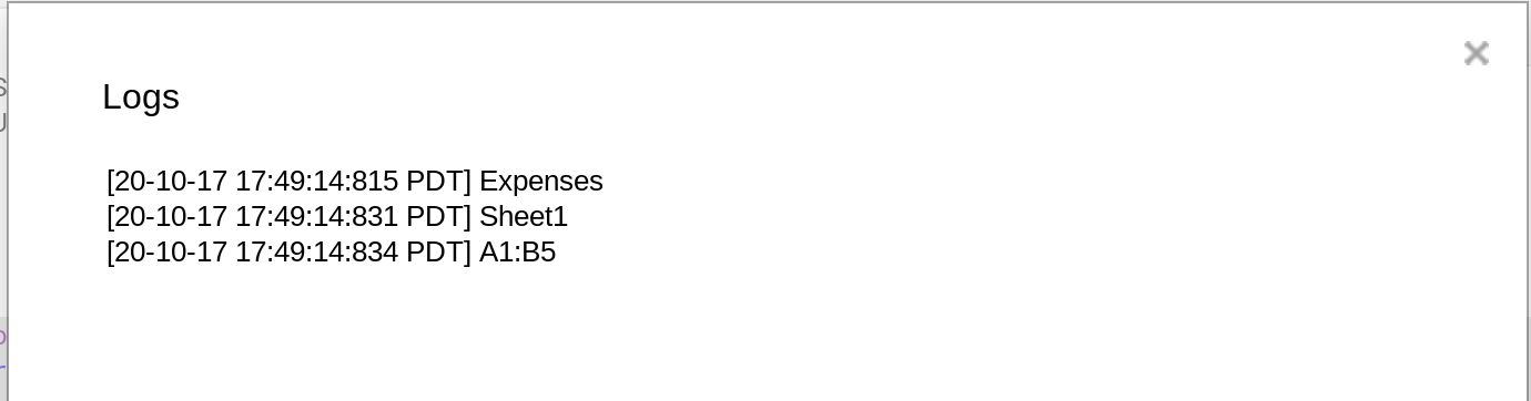
The logNamedRanges() function below, reads all the named ranges in the spreadsheet and logs their name, the name of the sheet that contains the range and the range's A1 notation.

function logNamedRanges() {
  var rangeList = SpreadsheetApp.getActive().getNamedRanges()
  rangeList.forEach(function (namedRange) {
    
    // Log the name of the range
    Logger.log(namedRange.getName());
    
    var range = namedRange.getRange();
    
    // Log the name of the sheet containing the named range
    Logger.log(range.getSheet().getName());
    
    // Log the named range's A1 notation
    Logger.log(range.getA1Notation());
  });
}

Conclusion

In this tutorial, you learned about named ranges in Google Sheets.

• Why should you use named ranges in Google Sheets?

• They make your formulas and scripts easier to understand. It is a lot easier to understand what =AVERAGE(StudentGrades) does than =AVERAGE(Sheet8!A1:A6).

• They make it easy to edit ranges that are used in multiple formulas and scripts. You can just edit the range associated with a name and all the formulas and scripts that use the named range will automatically begin using the edited range.

• How to create a named range in Google Sheets?

• Creating a named range using the Google Sheets UI

• There are two ways to create a named range using the Google Sheets UI:

• Select the range, right click and select Define named range

• Select Data —> Named ranges from the menu and then enter details.

• Creating a named range using Google Apps Script

• Use the setNamedRange() method of the Spreadsheet object to create a named range.

• How to use a named range in a Google Sheets formula?

• To use a named range in a formula, just use the name of the range instead of its A1 notation. So for example, use =SUM(Expenses) instead of =SUM(Sheet1!A1:A6).

• Working with named ranges in Google Sheets using Google Apps Script

• Reading data from a named range using Apps Script

• To read data from a named range, first reference the named range by using the getRangeByName() method of the Spreadsheet object. Then, read the values in the range by using the getValues() method.

• Writing data to a named range using Apps Script

• To write data to a named range, first reference the named range by using the getRangeByName() method of the Spreadsheet object. Then, write a two-dimensional array of values to the range by using the setValues() method.

• Note: the size of the array (i.e., the number of its rows and columns) must be the same as the size of the named range.

• Using named ranges with custom functions in Google Sheets

• You can use named ranges as arguments when calling a custom function from a cell in your spreadsheet. However, remember that Apps Script will retrieve the data contained in the named range and then pass this data to the function. The custom function will not know which range this data is coming from (or if it even is even coming from a range in your spreadsheet).

• Reading all the named ranges in a Google Sheets spreadsheet

• Use the getNamedRanges() method of the Spreadsheet object to get all the named ranges in your Google Sheets spreadsheet.

Thanks for reading!