Range in Google Sheets

This tutorial will introduce you to the concept of a range in Google Sheets. You'll learn about what ranges are and how to use them. You'll also learn about named ranges and the benefits of using them.

What is a range?

A range represents a single cell or a group of adjacent cells in your spreadsheet. Every time you work with data in a spreadsheet, you're likely using one or more ranges.

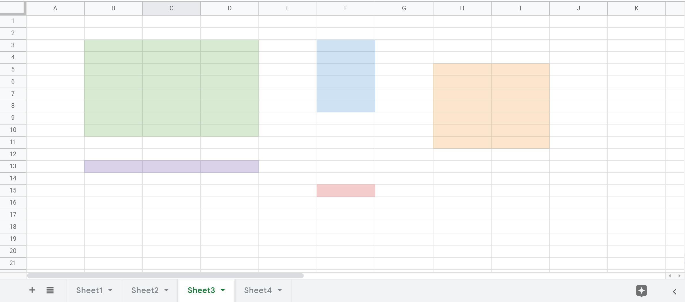
The screenshot below shows 5 different ranges in Sheet3 of your spreadsheet.

How to reference a range in a Google Sheets formula?

To reference a single cell in a formula, use the name of the sheet followed by an exclamation mark, the column and finally the row.

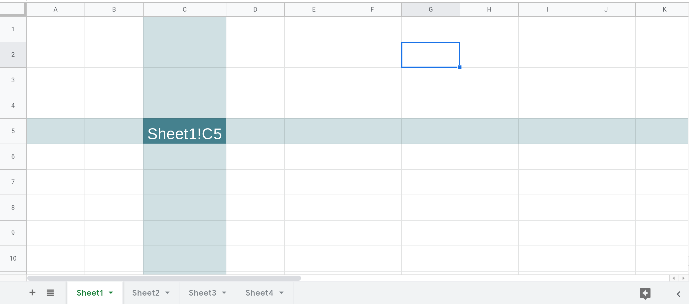
A cell that is in Sheet1 at the intersection of column C and row 5 will have the following reference:

Sheet1!C5. This type of reference is known as A1 notation.

To reference a range composed of a group of adjacent cells, we'll need to specify the two cells that are at corners of any diagonal within the range. Typically, the cells that are at the top left and bottom right corner are the ones that are specified.

The screenshot below displays multiple ranges (the ones that have been colored) and in each case the top left and bottom right cells have been filled with a darker color.

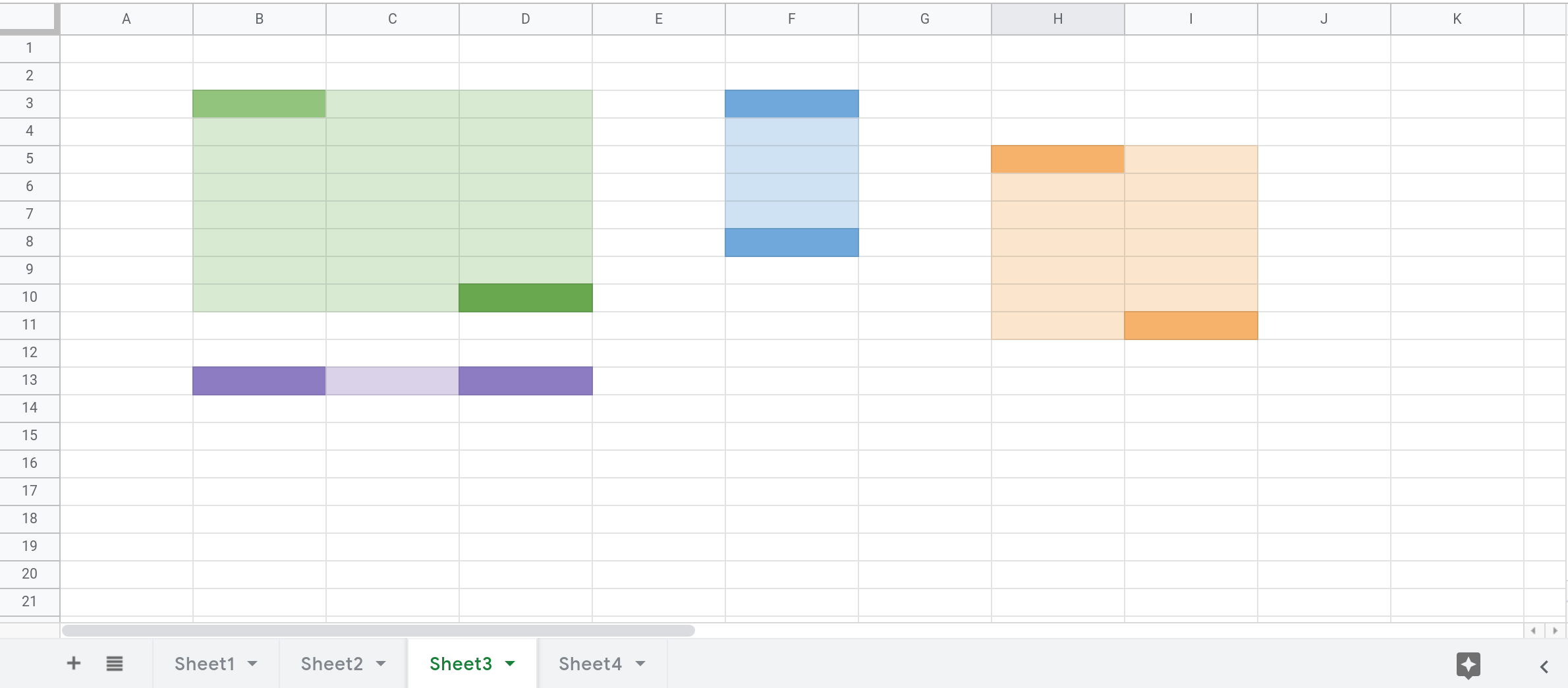
To reference a group of cells in a formula, use the name of the sheet followed by an exclamation mark, the column of the top left cell, its row, a colon, the row of the bottom right cell and finally its column.

For example, the below references correspond to the ranges highlighted in the above screenshot.

• Range colored green: Sheet3!B3:D10

• Range colored blue: Sheet3!F3:F8

• Range colored: purple: Sheet!B13:D13

• Range colored orange: Sheet3!H5:I11

You can also define ranges that reference entire rows or columns:

• All rows in one column: Sheet3!B:B (use the column name twice and omit the row numbers)

• All rows in multiple adjacent columns: Sheet3!B:D (use the names of the first and last column in the range and omit the row numbers)

• All columns in a single row: Sheet3!2:2 (use the row number twice and omit the column names)

• All columns in multiple adjacent rows: Sheet3!2:10 (use the numbers of the first and last row in the range and omit the column names)

How to use a range in a Google Sheets function?

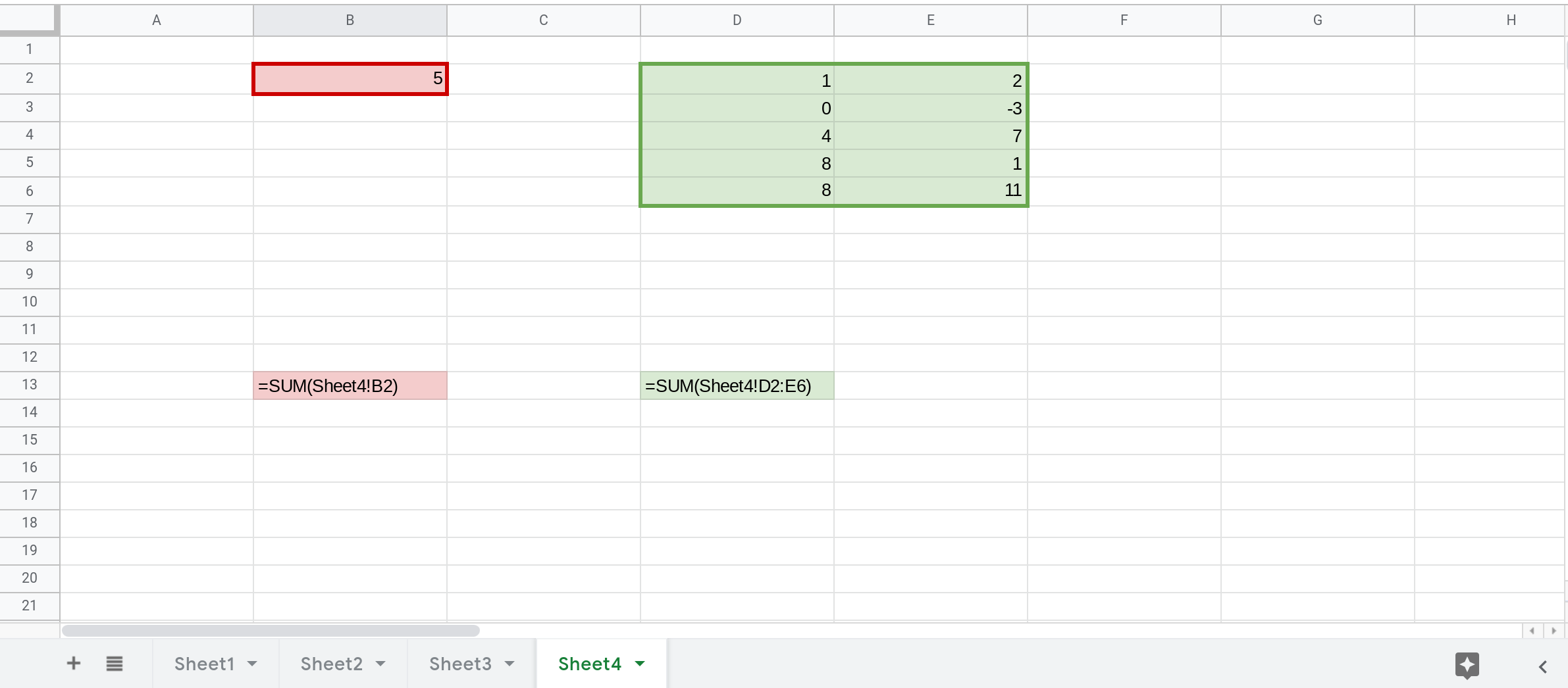
To use a range in a function, just use the range's reference. For example, in order to calculate the sum of values in the range Sheet4!D2:E6, use the formula =SUM(Sheet4!D2:E6). To sum values in just a single cell, say Sheet4!B2, use =SUM(Sheet4!B2).

Named ranges in Google Sheets

In Google Sheets, you can assign a name to a range. Once you do this, you can use the name of a range instead of its reference in formulas and scripts.

There are several ways to create a named range:

1. Select Data —> Named ranges and enter the name and reference.

2. Select a range in the spreadsheet, right click and select Define named range to give it a name.

3. Create a named range by using Google Apps Script.

You can also create named ranges using Google Apps Script. The code below shows you an example of how to do that.

function createNamedRange(name, range) {
  SpreadsheetApp.getActive().setNamedRange(name, range);
}

Once you create a named range, you can use it in formulas and scripts by using its name. So, instead of Sheet2!A1:C6, you can use the range's name like this: StudentGrades.

Using named ranges has several benefits:

• Formulas and scripts will become more readable because the name of the range will help users understand the type of data contained in it. For e.g., StudentGrades is a lot more descriptive than Sheet2!A1:C6.

• When you make changes to a named range, all the formulas and scripts will immediately begin using the updated range.

Conclusion

This tutorial covered the basics of working with ranges in Google Sheets. You learned how to:

• Reference a range in a Google Sheets formula

• Use a range in a function

• Create and use named ranges

Thanks for reading!