How to make a Table in Google Sheets?

Most of the business world runs on spreadsheets and many of these spreadsheets contain tabular data. Therefore, one might assume that spreadsheet software comes with native support for working with these tables effectively and efficiently. Sadly this isn't true!!

In this tutorial, I will show you how you can use formulas and other features in Google Sheets to build some desirable features that will make your tables less error prone and more effective at conveying information.

What does having native support for tables in spreadsheets even mean? Isn't the spreadsheet itself basically just one large table?

Let me try and explain what I mean by native support for tables with a few examples.

#1 Formatting for visual presentation.

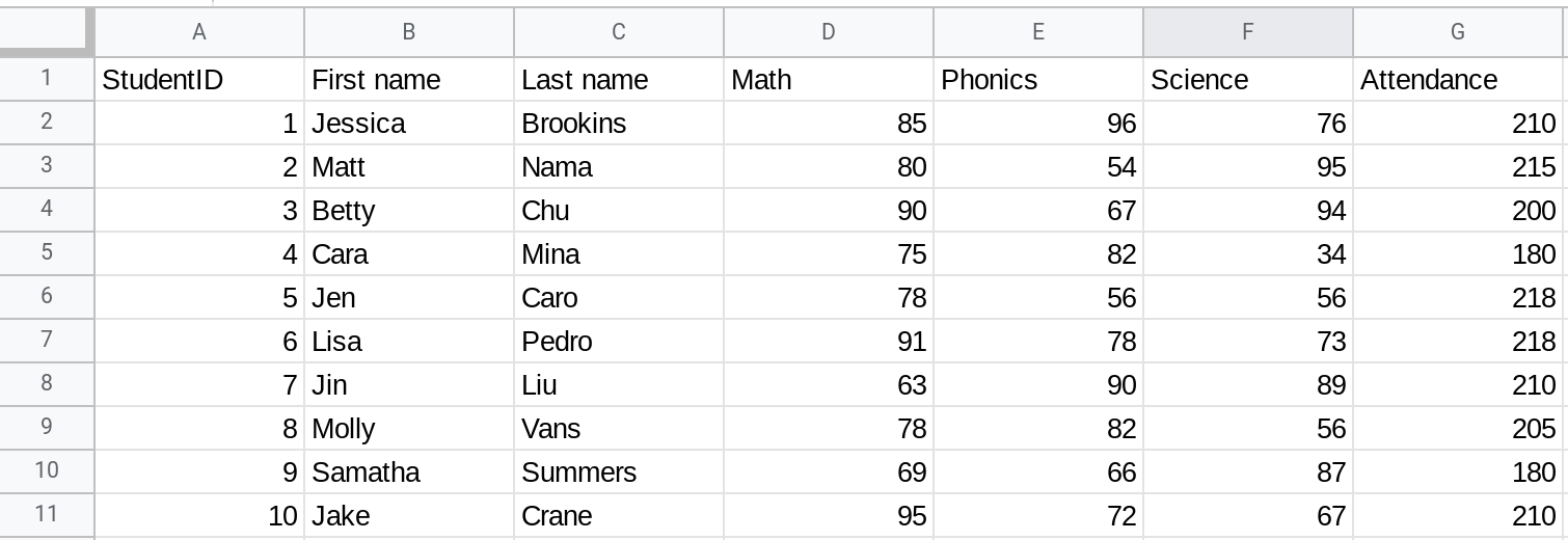
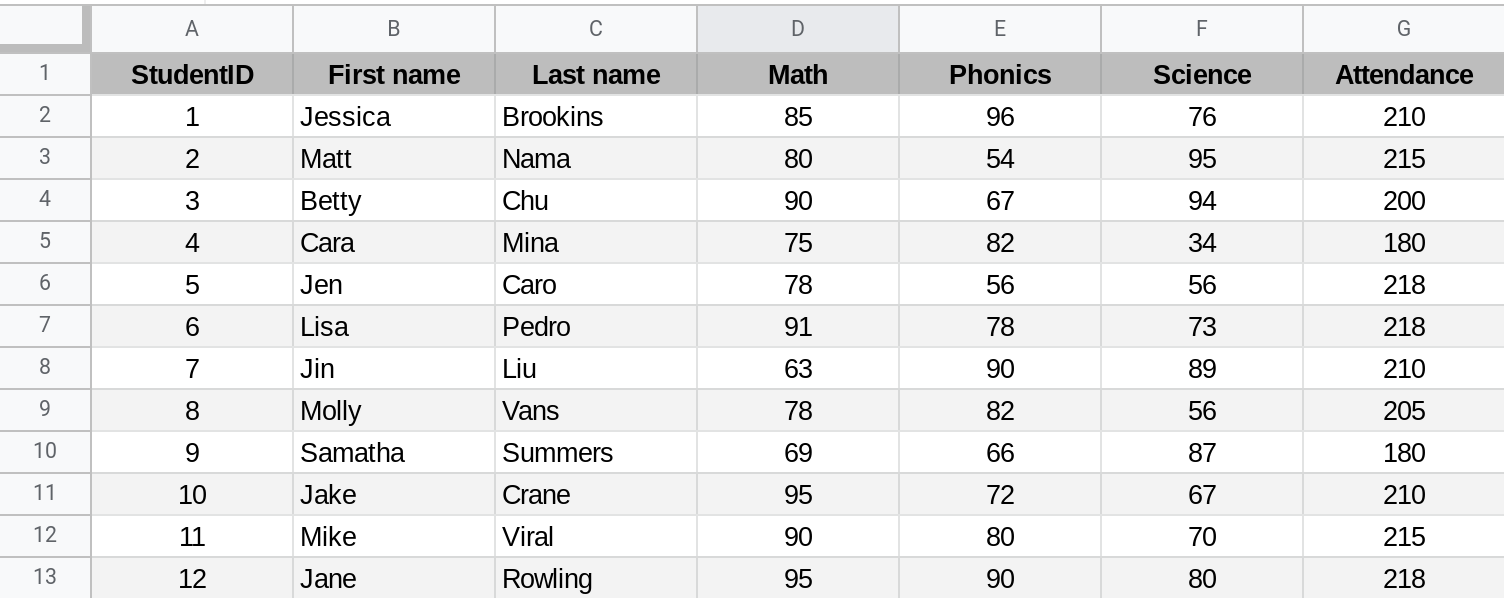
Let's say you have a table in Google Sheets that contains information about 10 students in your class. Here is how that data looks upon entering it:

Now, if you want to format it to make it look 'presentable', there isn't a simple 'one-click' mechanism to do that. As you'll see later in this tutorial, you could do a couple of things to make it look nice but you'd have to do this manually and repeat these steps every time you create a new table in Google Sheets.

#2 Filtering and sorting

A very common use case when working with tables is filtering and sorting their contents to make sense of the data they contain. Again, you can certainly do this manually in Google Sheets but there is no way to tell the spreadsheet that these 11 rows and 7 columns are a table and have this filter be created automatically.

#3 Automatically compute aggregate metrics (aka the "Totals" row)

This is probably the most important requirement and the one that I wish was supported by all spreadsheet software.

Let me explain the problem first. Let us say you have a table with three rows. You create a "Totals" row where you add up numbers in the three other rows. Now suppose you insert two new rows into the table. Unless you carefully structure the formulas in the totals row, they might still be adding numbers from just the three original rows instead of the five current ones.

Ideally, the spreadsheet software would automatically ensure that the totals reflected the data in the table. Unfortunately it is left to us, the users of the spreadsheet, to double and triple check the results produced by spreadsheet analysis. It is not surprising that errors creep into analysis performed using spreadsheets.

The good news is that Microsoft Excel does have a "Tables" feature and has good native support for working with tables. In this tutorial I will show you how to replicate some of this functionality in Google Sheets.

Prerequisites

This tutorial assumes that you are familiar with using Google Sheets. In particular, it assumes that you are familiar with the following concepts in Google Sheets:

• Formatting data (how to format text, cell backgrounds, etc.)

• Creating filters

• Creating named ranges

• Functions (especially: OFFSET, ROWS, COLUMNS, MATCH, INDIRECT, CONCAT)

5 steps to make a table in Google Sheets

• Step 1 — Create a Google Sheets spreadsheet with tabular data and format the data

• Step 2 — Create a filter so users can easily filter rows in the table

• Step 3 — Make the totals row auto-update aggregate metrics when rows are inserted into or removed from the table

• Step 4 — Name your table by creating a named range for it

• Step 5 — Test entering rows in your table

Step 1 — Create a Google Sheets spreadsheet, enter tabular data in it and format the data

The first step is to open a Google Sheets spreadsheet that contains some tabular data. If you don't have an existing spreadsheet you can use, simply create a new one and enter some test data into it that you can use.

If you want, you can copy and paste the table below into your spreadsheet.

The next step is to format this data.

Best practices for formatting tables in Google Sheets

Here are some best practices for formatting tabular data so it looks professional and makes it easy for both you and others to read and work with the data.

Format the header row in your table

Ensure that you bold and center the values in your header row. If the number of rows in your spreadsheet exceeds your screen's view port (meaning you need to scroll to view all the rows), try to ensure the header row is the first row in the sheet and freeze it. This way you'll be able to see the header row even when you're scrolling down.

Align text in your table

In general, Google Sheets has good defaults for text alignment but If your column contains numeric values that do not represent numbers then format them as text. In some cases you might want to center them (e.g. the numbers are serial numbers) and in other cases you might want them left aligned (e.g. the numbers are large and represent employee IDs in a Fortune 500 company).

Format numbers in your table

If you have columns containing monetary values or dates (yes Google Sheets stores dates as numbers!), then ensure you format these columns accordingly.

For example, users of your spreadsheet should be able to figure out if a number represents a monetary value and the currency it is denominated in. Seeing $20 tells me that the value in that cell represents 20 US dollars. Just seeing the number 20 will not convey this same information.

Use alternating colors to make adjacent rows stand out clearly

Which of the two tables below is easier to read? A or B?

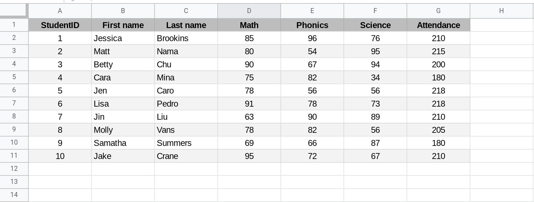
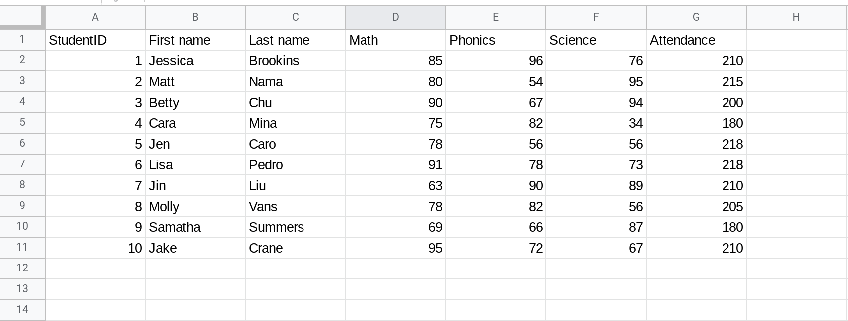
• [A]: A table where rows are formatted using alternating colors

  

• [B]: A table where rows aren't formatted using alternating colors

  

The alternating colors in Table A make it easier to quickly scan the rows in the table. The contrast between adjacent rows makes it easier to stare at a large number of rows.

Here is a video that demonstrates how to apply some of the above best practices:

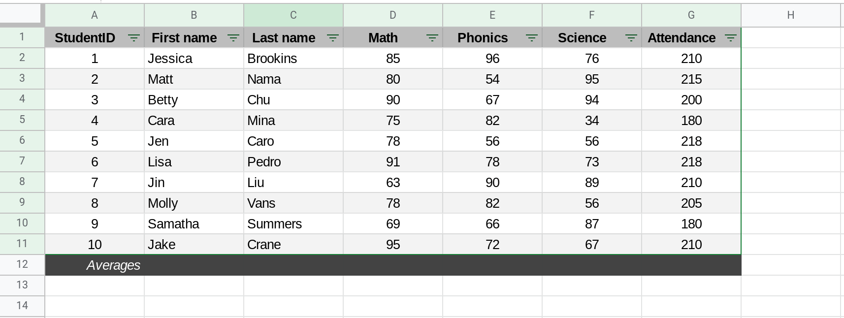
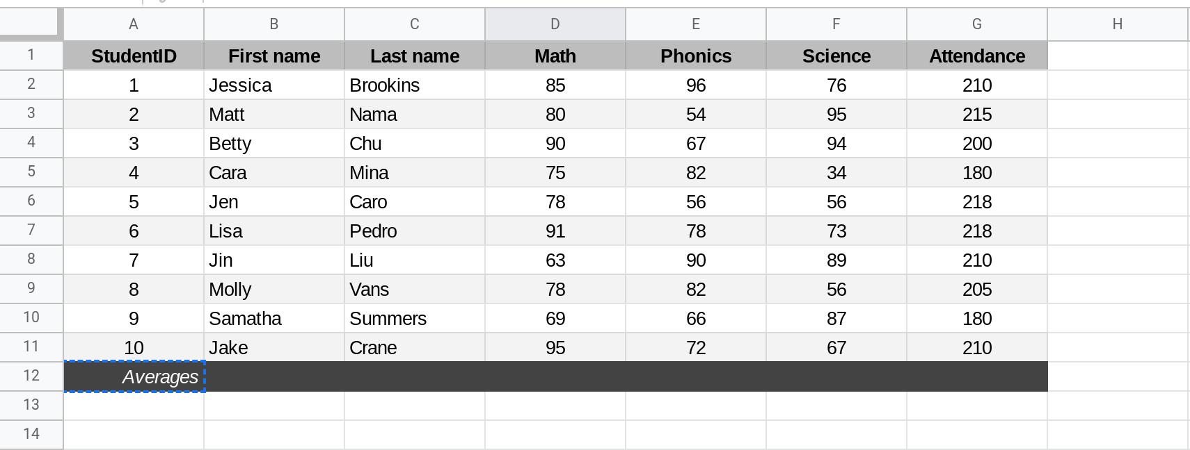
Add a totals row to your table to display aggregate metrics

Insert a row at the bottom of your table to compute aggregate metrics based on the values in your table. In this example, we will use this row to compute and display average scores and the average attendance for students in the class.

We will come back to this row in step 3 to populate it.

Step 2 — Create a filter so users can easily filter rows in the table

A common use case when working with tables is filtering rows based on the values in specific columns. For example, you might want to quickly see which students are doing poorly in Math. You can filter the table to only show students whose math score is less than 50.

To create a filter select all the rows in your table except the totals row. Then select Data from the menu and select Create filter.

Step 3 — Use the INDIRECT function to make the totals row auto update whenever rows are inserted into or removed from the table

Suppose you have the following table in your spreadsheet:

If you insert a row in the above table, the formula in the totals row may no longer be correct since it may not include the row (highlighted in red below) that you just inserted.

Sometimes Google Sheets will correctly update the formula in the totals row to also include the newly inserted row but a better way to do this is to structure your formulas to be robust and account for future addition or deletion of rows.

Now what if we could make the AVERAGE() function be applied to a range that starts at cell B2 and ends at the row that is just before the totals row?

So instead of =AVERAGE(B2:B4), what if we could do something like =AVERAGE(B2:B<PREVIOUSROW>)? Here we'd want "<PREVIOUSROW>" to dynamically update to always be the row that is the one just before the totals row.

One way to achieve this is by using the INDIRECT() function.

The INDIRECT() function takes the address of a cell as a string and returns a reference to it. So INDIRECT("B4") will return a reference to the cell B4 and =INDIRECT("B4") has the same effect as =B4.

Now, the function ROW() returns the row number of the current cell therefore ROW()-1 is the number of the row that is just before the current row. The function CONCAT() is used to concatenate two values together into a single string. So CONCAT("B",ROW()-1) will return a string that represents the cell in column B that is on the previous row.

Therefore, INDIRECT(CONCAT("B",ROW()-1)) is a reference to the cell in column B that is on the previous row. This is exactly what we need to implement B<PREVIOUSROW>.

In the totals row, if we replace =AVERAGE(B2:B4) with =AVERAGE(B2:INDIRECT(CONCAT("B",ROW()-1))) then we will ensure that no matter how many rows are inserted into the table, the average value in the totals row will be based on the range that begins at row 2 in column B and ends at the row just before the totals row. Now we are no longer dependent on Google Sheets doing the right thing when users insert or delete rows, the formula we are using itself enforces the desired behavior.

The video applies this approach to the table we have been creating in this tutorial.

Step 4 — Name your table by creating a named range for it

Another best practice when working with tables in Google Sheets is to name the table by creating a named range. This will let you reference the table elsewhere in your spreadsheet by using its name.

When creating a named range for a table include the header row but do not include the totals row. This is because you might want to perform some other computation on the table's contents using this named range and including the totals row (which was itself computed) in it will lead to incorrect results.

In the above video, I use the name students for the table. So, suppose I now want to add up the attendance of each student, I can simply say:

=SUM(OFFSET(students,1,6,ROWS(students)-1,1)).

How does the above formula work?

The OFFSET() function in Google Sheets returns a range reference that is shifted a specified number of rows and columns from a starting cell reference.

The syntax for the OFFSET() function from the Google Sheets documentation is:

OFFSET(cell_reference, offset_rows, offset_columns, [height], [width])

What does the above syntax mean? Let's use a simple table as an example to learn how the OFFSET() function works.

Suppose we have the following table in Google Sheets and let's say the table (i.e. the range A1:B4) is named math_grades.

Now, let us consider the formula =OFFSET(A1,1,2,1,2).

The first parameter A1 is the cell to start from.

The second parameter indicates how many rows to move (i.e. offset) by. If this value is positive we move downwards and if it is negative we move upwards.

Here the value is 1 (which is positive) so we move downwards to the next row.

The third parameter indicates how many columns to move (i.e. offset) by. If this value is positive we move to the right and if it is negative we move to the left.

Here the value is 2 (which is positive) so we move right by 2 columns. Since the table only has two columns, when we move two columns right from the first column, we move outside the table to column C.

The last two columns specify the height and width of the range to return starting from the cell position specified by the offsets. Since these values are 1 and 2 respectively, the formula =OFFSET(A1,1,2,1,2) will return a range that contains one row and two columns starting from the cell C2.

In this example, =OFFSET(A1,1,2,1,2) results in the range C2:D2.

Working with tables in Google Sheets using the OFFSET() function

Now that you have learned how to work with the OFFSET() function, let us go back to the original formula =SUM(OFFSET(students,1,6,ROWS(students)-1,1)) and try to understand it.

The named range students represents the following table:

As we saw previously, the first parameter in the OFFSET() function specifies where to start. Here, the first parameter in OFFSET(students,1,6,ROWS(students)-1,1) is actually a named range and not a cell. Therefore, the starting point will be the first cell in that range (students), which is cell A1.

The second parameter specifies the number of rows to offset. Here it is 1, which is positive so we move downwards by a row.

The third parameter specifies the number of columns to offset. Here it is 6, which is positive so we move right by 6 columns which gets us to cell G2.

The last two parameters specify the height and width of the range to return. Here these are ROWS(students)-1 for height and 1 for width.

Now, ROWS(students) returns the number of rows in the range named students, which is 11 rows. So ROWS(students)-1 is 10. Therefore, the formula will return a range starting from cell G2 that has a height of 10 rows and width of 1 column.

This is exactly the range that you would want to SUM if you wanted to compute the total attendance (in number of days attended) across all students in the class.

Suppose you wanted to SUM some other column in the table, all you need to do is change the column offset (6) to the right value. So to SUM the math grades, change 6 to 3 in the formula.

=SUM(OFFSET(students,1,3,ROWS(students)-1,1))

Notice that you don't need to worry about how many rows are in the table. You only need to worry about the position of the column you care about within the table.

The one place where Microsoft Excel does a better job than Google Sheets is you can also refer to a column in a table by using its header. You can do that in Google Sheets too by creating a named range for every column in the table but that can be cumbersome if you have lots of columns in your table.

A better approach is to use the MATCH() function to dynamically figure out which column in the table has a given header. So instead of remembering that fourth column contains math grades, you can use the formula a formula to figure this out automatically:

MATCH("Math",OFFSET(students,0,0,1,COLUMNS(students)),0)

Now, the formula =SUM(OFFSET(students,1,3,ROWS(students)-1,1)) can be made even more robust:

=SUM(OFFSET(students,1,MATCH("Math",

OFFSET(students,0,0,1,COLUMNS(students)),0)-1,

ROWS(students)-1,1))

If you now want to compute the SUM of all Phonics scores, all you need to do is replace "Math" in the above formula with "Phonics". That's it!

Step 5 — Test entering rows in your table

The final step is to test entering new rows in your table to confirm that the totals row is being computed correctly. The video below demonstrates this.

Here are some more ideas for improvements that you can make to the table:

• Use the ROUND() function to round values wherever applicable.

• Using conditional formatting to flag students with very low test scores.

Conclusion

In this tutorial, I showed you how to create tables in Google Sheets to convey information effectively while also minimizing the potential for errors.

Hope you found this tutorial helpful. Thank you for reading.