Checkboxes in Google Sheets ☑️

You can use checkboxes to make your Google Sheets spreadsheet interactive. For example, in this tutorial, you'll learn how to build a simple To Do list application 📋 in your spreadsheet by using checkboxes and conditional formatting.

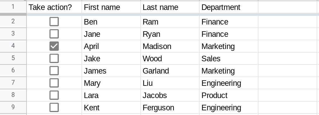
Another common use case for checkboxes in Google Sheets is making it easy for users to select specific rows to be processed by a Google Apps Script script. For example, consider the following table containing information about employees.

Column A in the above table indicates whether or not some action needs to be taken for each row. One approach could be to enter "Y" to indicate the rows that should be processed.

This can be made seamless by using checkboxes. When the checkbox in a row is checked, it indicates that the script should process that row.

There is SO much that you can do with checkboxes to add interactivity to your Google Sheet. In this tutorial we will explore one use case, and in subsequent tutorials (like this one) we will explore many more.

Prerequisites

This tutorial assumes that you are familiar with the basics of Google Sheets:

• Ranges in Google Sheets.

• Using conditional formatting rules in Google Sheets.

• Data validation and how to use it.

What you will learn in this tutorial

This tutorial covers the following topics:

• How to insert checkboxes into a Google Sheets spreadsheet?

• A checkbox is just a data validation that is applied to a range in your spreadsheet.

• How to assign custom values to the checked and unchecked states of the checkbox?

• Building a simple To Do list application in Google Sheets by using checkboxes and conditional formatting.

How to insert checkboxes into a Google Sheets spreadsheet?

To insert checkboxes manually, first select the range and then select Insert —> Checkbox from the menu.

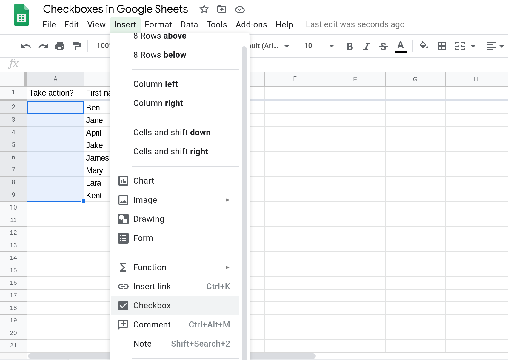
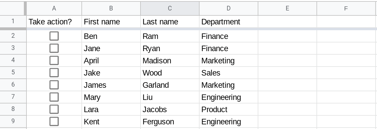
You should now see checkboxes in the range that you selected.

A checkbox in Google Sheets is just a data validation with two states: Checked and Unchecked

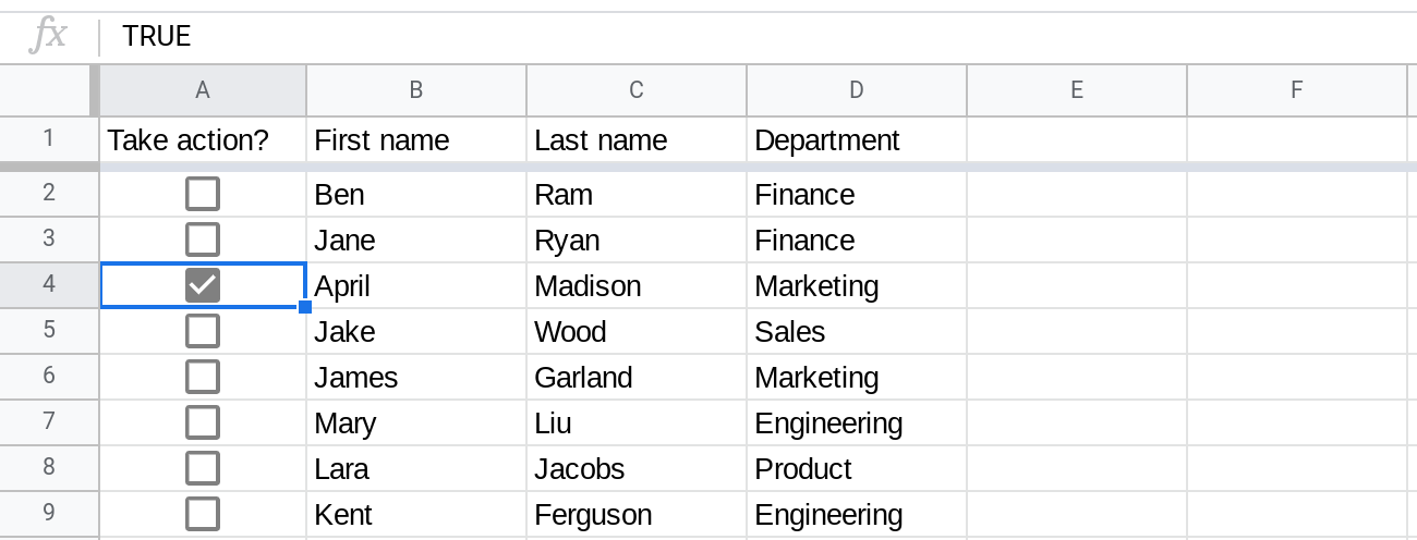
A checkbox in Google Sheets is implemented behind the scenes as a data validation. When you insert a checkbox in a cell, that cell can take on one of two values. By default, the value will be TRUE when the checkbox is checked and FALSE when it is unchecked.

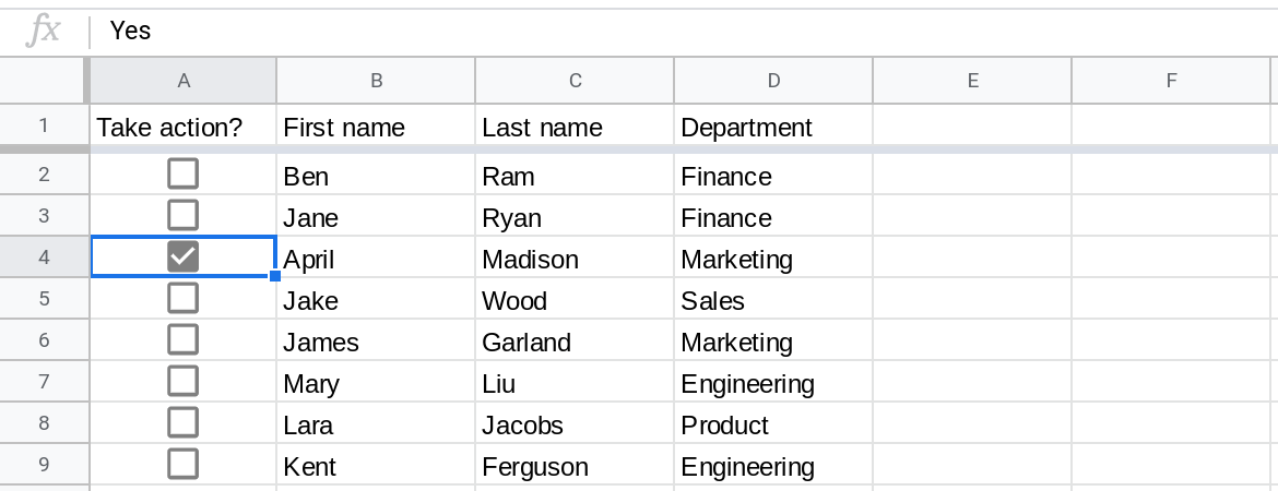
Below is a screenshot that shows the value in cell A4 to be TRUE because the checkbox is checked.

In fact, since a checkbox is implemented as a data validation, you can also insert a checkbox by adding validation to a range.

To try this, first select the range, then select Data —> Data validation.

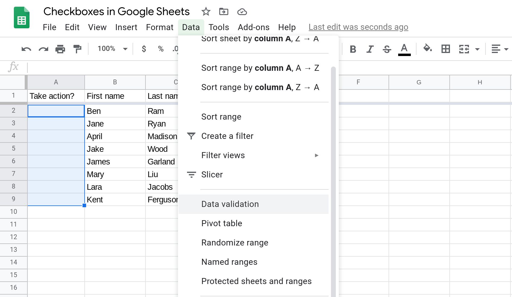
Choose Checkbox as the criteria type and select Save.

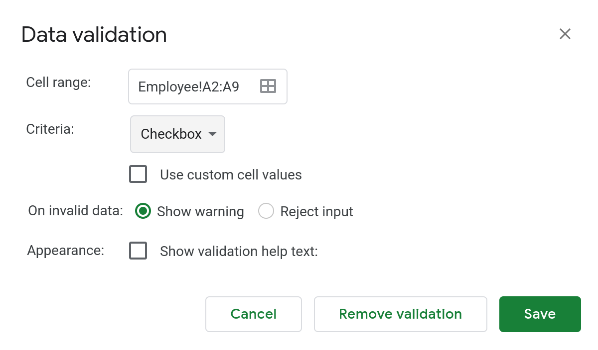
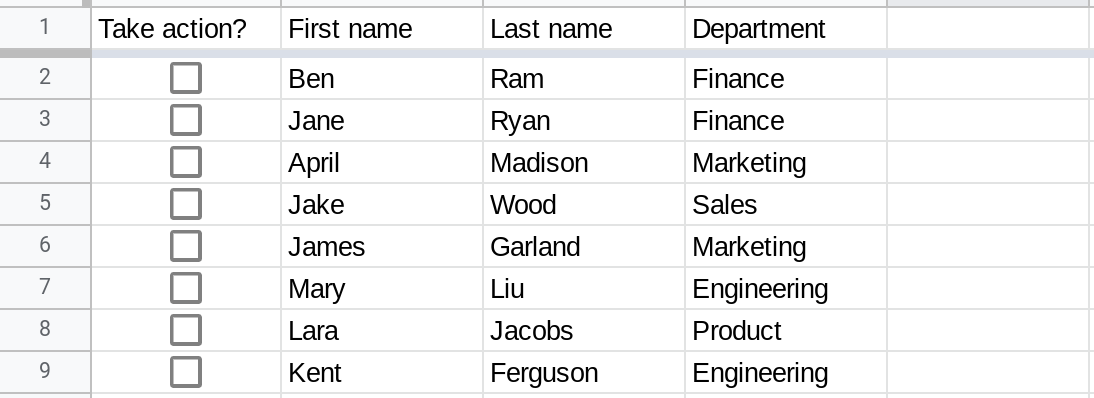
You should now see checkboxes in the range that you selected.

Assigning custom values to the checked and unchecked states of a checkbox in Google Sheets

By default, the checked and unchecked values of a checkbox are set to TRUE and FALSE respectively. However, you can override this and set custom values for both states.

To do this, select the Use custom cell values checkbox when setting up the data validation and enter the values for the two states. In the screenshot below, I entered "Yes" for the checked state and "No" for the unchecked state.

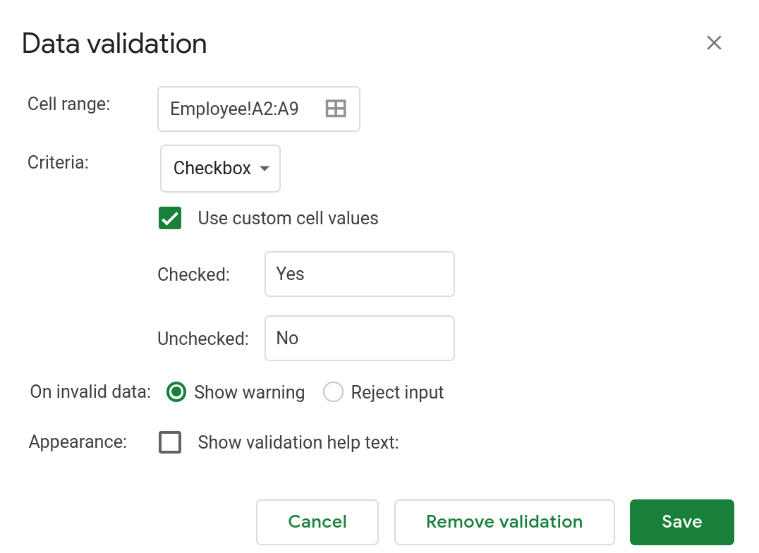
The cell A4 in the screenshot below is set to the value Yes (instead of TRUE) since the checkbox in that cell is checked.

Building a To Do list application in Google Sheets by using checkboxes and conditional formatting 📋

Google Sheets constantly amazes me since you can build so many useful applications

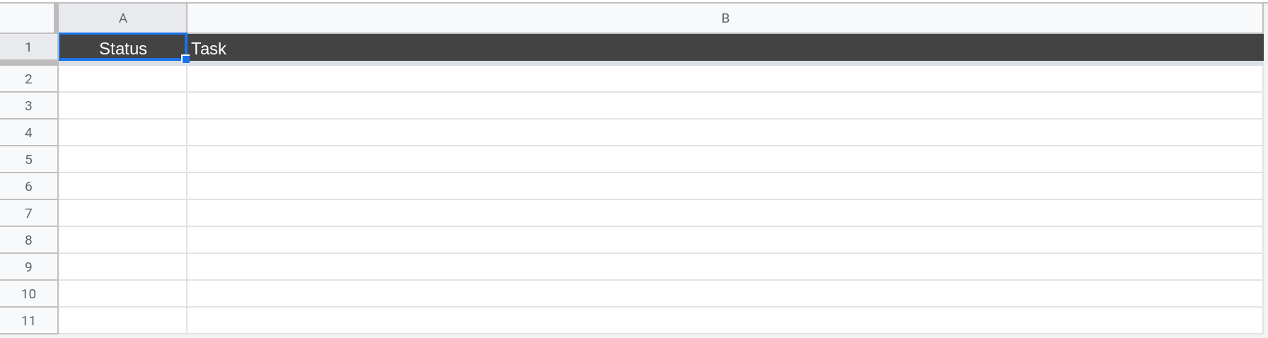
Step 1 — Create a spreadsheet with two columns: status and task

In the spreadsheet below, I'm using column A for recording the status of a task and column B for a description of the task.

Step 2 — Add data validation to the status column

The next step is to insert checkboxes into the spreadsheet in column A.

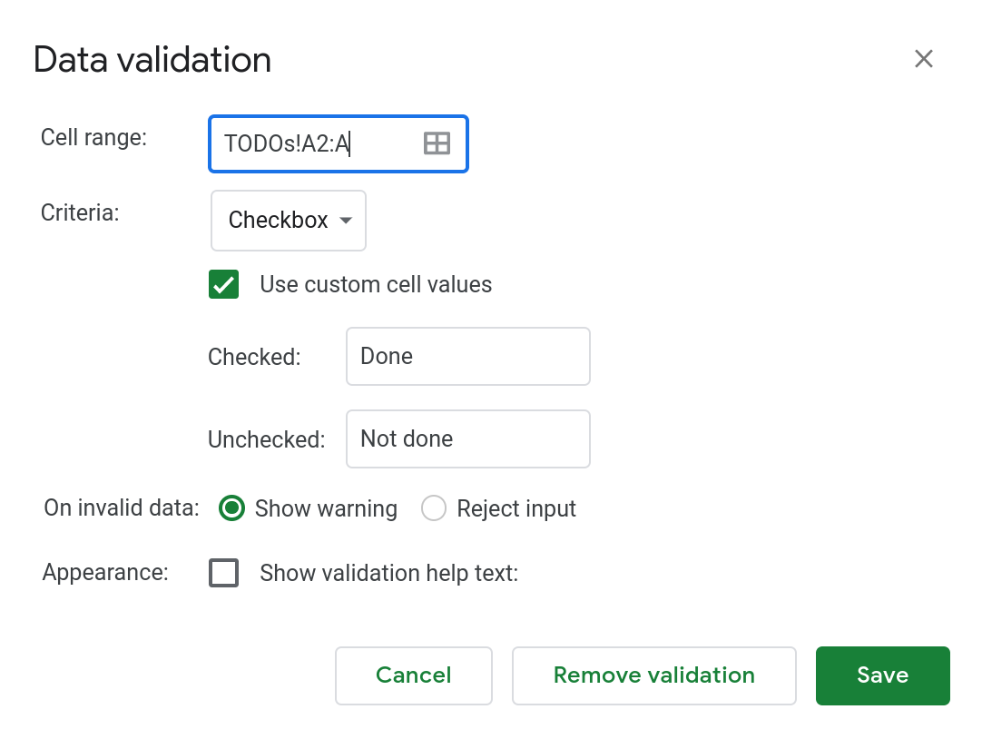
• Select column A starting with cell A2 (not A1 since you don't want a checkbox inserted into the header row).

• Then select Data —> Data validation from the menu.

• Then edit the Cell range to ensure the range is A2:A (notice that there is no row number at the end). This will ensure that the data validation is automatically applied to any new rows that you insert into your spreadsheet.

• Select Checkbox as the criteria.

• Select Use custom cell values and add Done for the Checked state and Not done for the Unchecked state.

• Select Save to add the validation.

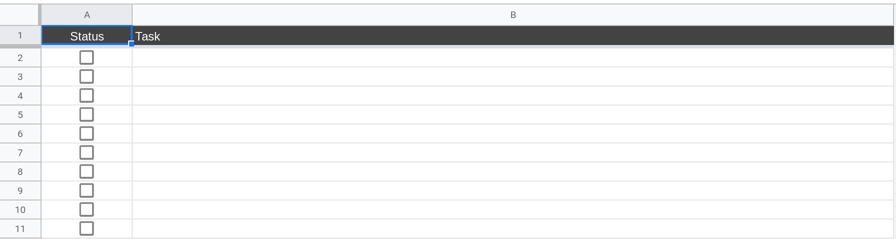
You should now see checkboxes in column A.

Step 3 — Add conditional formatting to your spreadsheet

The final step to complete the To Do application is to add conditional formatting to mark tasks as Done when the checkbox is selected.

• First, select all the rows other than the header row in your spreadsheet.

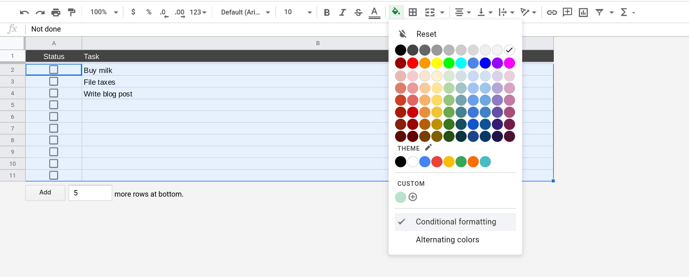
• Then select Fill color from the toolbar and select Conditional formatting.

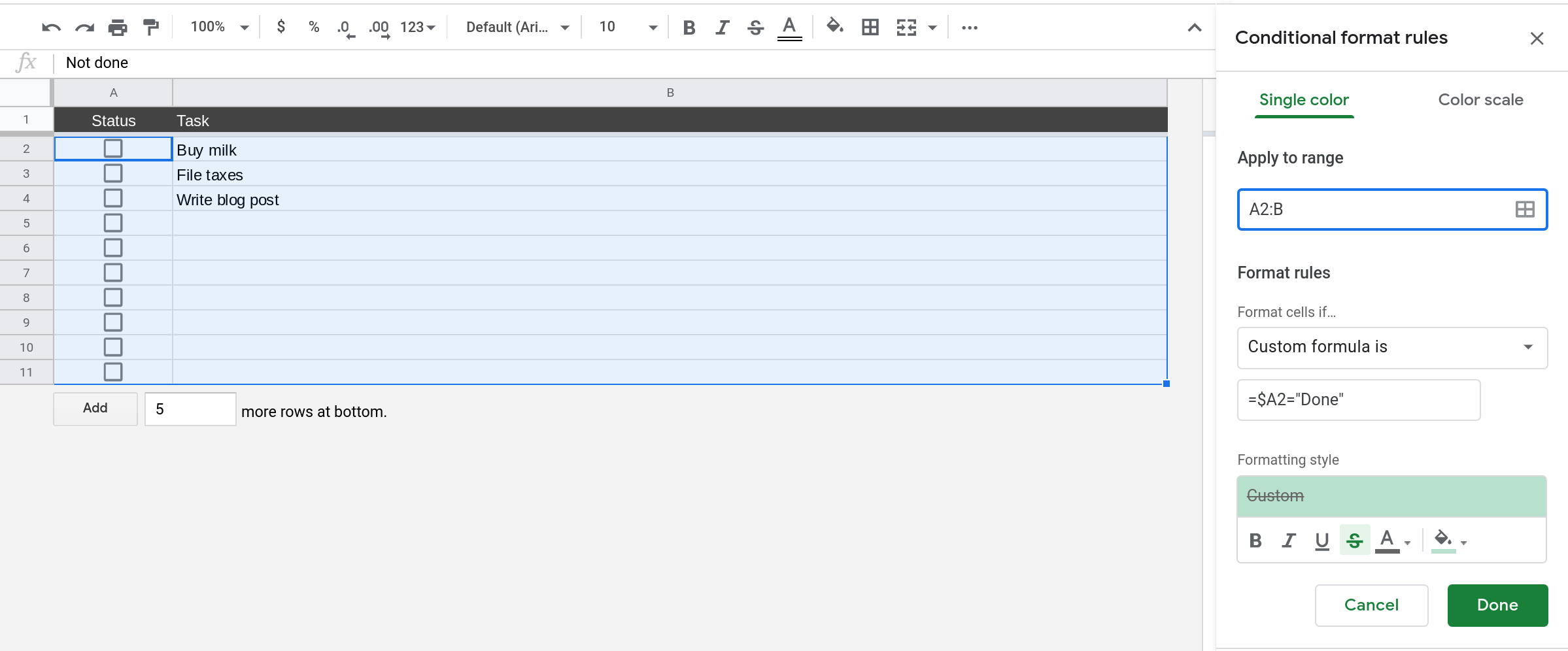
• Enter the range the formatting should be applied to as A2:B (notice there is no row number at the end).

• Select Custom formula as the formatting condition and enter =$A2="Done" as the custom formula.

• Select the formatting style for your completed tasks. I chose to highlight completed rows in green with dark gray text that is crossed. Somehow, seeing a To Do crossed out gives me extra joy 😊!!

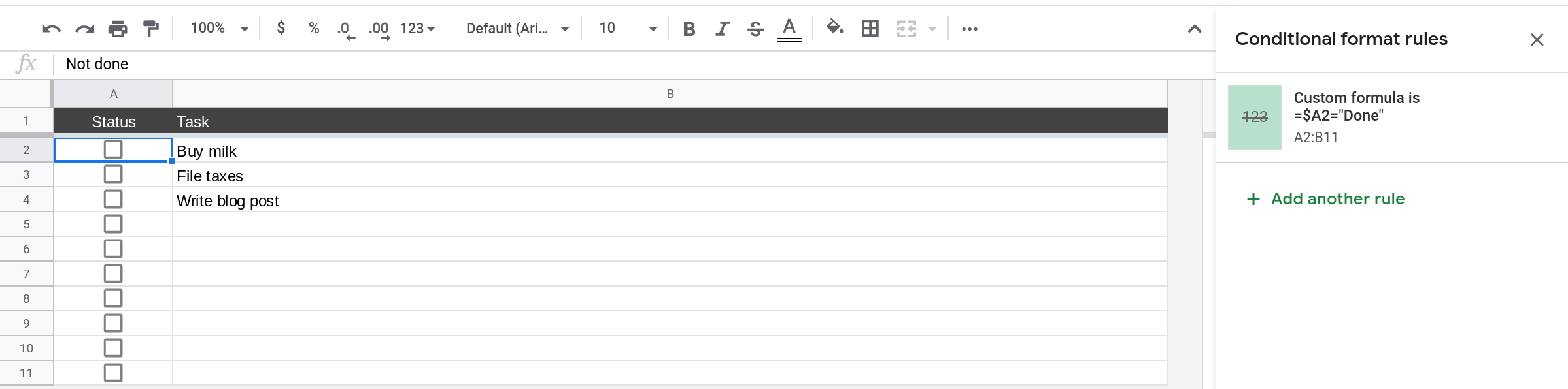
• Finally, select Done to add the conditional formatting to the range.

When you select Done, you should see a summary of the conditional formatting rule that you specified in the sidebar.

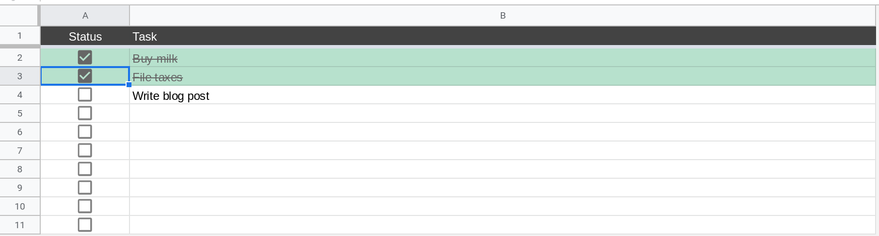
Now whenever you mark a task as done, you should see the row's formatting update per the conditional formatting rule you specified.

That's it! In just a few minutes you built a simple To Do application using Google Sheets. Isn't that awesome?

Conclusion

In this tutorial, you learned how to use checkboxes in Google Sheets. You also learned how to build a simple To Do list application using just checkboxes and some conditional formatting.

If you enjoyed this tutorial and you want to learn more, I've got you covered! Please check out my tutorial on how to work with checkboxes in Google Sheets using Google Apps Script.

Thanks for reading!