Hide rows based on cell value in Google Sheets using Apps Script

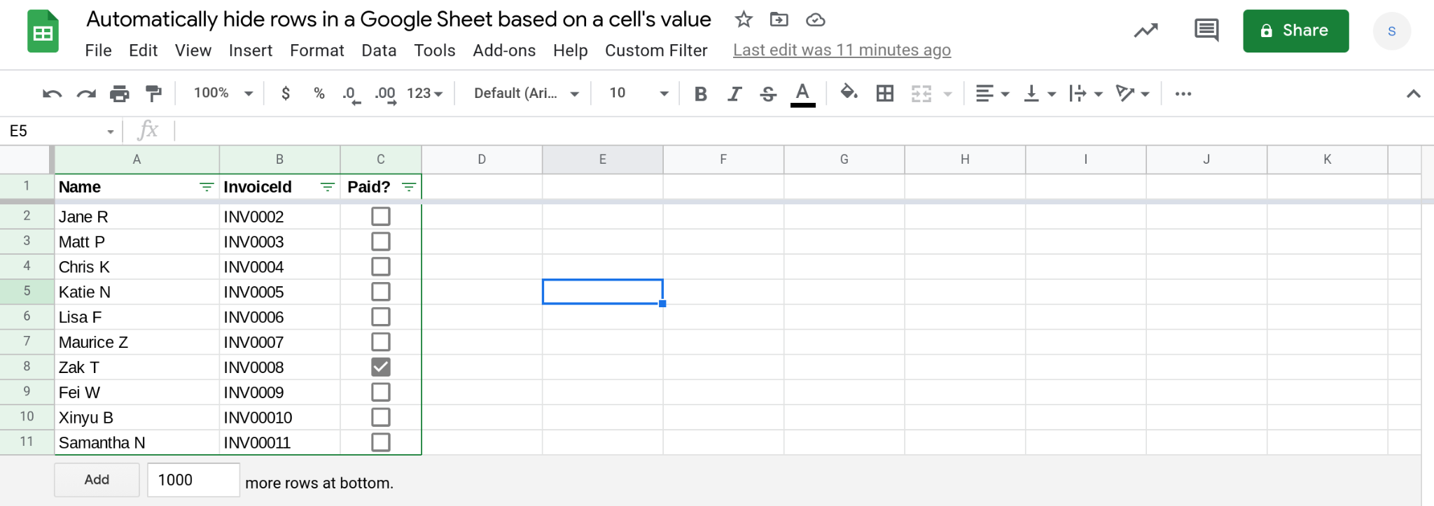
In this tutorial I will show you how to hide rows in Google Sheets based on cell value. In the spreadsheet below, there are three columns: Name, InvoiceId and Paid. The column Paid can contain either "Y" or "N" and we've inserted checkboxes with custom values to make it easy to set the payment status of each invoice. Our objective is to make it easy to hide invoices that have already been paid. That is, we want to hide rows where the checkbox is checked.

There are a few different ways to achieve this. For e.g., you can create a filter or a filter view in your sheet. However, the disadvantage of these methods is that it can be cumbersome to hide or unhide rows as you make changes to your sheet. The video below demonstrates this.

In the video above, despite setting up a filter, it isn't easy to hide rows that are newly marked as paid. You have to select the filter settings and then select Ok each time you want the filter to process new changes in your spreadsheet.

In this tutorial, I will show you how to make this workflow more seamless by using Apps Script. We will build a custom menu called "Custom Filter" with two menu items: (1) Filter rows, and (2) Show all rows. Selecting Filter rows will hide all rows that are marked as paid. Selecting Show all rows will unhide all rows in your spreadsheet. The video below demonstrates this.

Prerequisites

This tutorial assumes that you're familiar with the following concepts:

• Basics of working with Google Sheets

• Basics of working with Google Apps Script

• Creating custom menus in Google Sheets

• The For loop in Google Sheets

• Reading data from a range in Google Sheets

4 steps to hide rows based on cell value in Google Sheets using Apps Script

• Step 1 — Create your Google Sheets spreadsheet

• Step 2 — Create a function to filter rows based on the value in a specific column

• Step 3 — Create a function to show all rows

• Step 4 — Create a custom menu to make it easy for users to run these functions

Step 1 — Create your Google Sheets spreadsheet

The first step is to open your spreadsheet or create a new one. I'm using a spreadsheet with 3 columns: Name, InvoiceId and Payment status (Paid?).

Our goal is to hide rows where the cell in a given column has a specific value. In this tutorial, we will hide rows where the payment status is set to "Y" (i.e., the checkbox is checked).

Once you have your spreadsheet ready, the next step is to write some code using Apps Script. Open the Apps Script code editor by selecting Tools —> Script editor and then proceed to Step 2.

Step 2 — Create a function to filter rows based on the value in a specific column

Create a function called filterRows() that will hide rows in your sheet where the 3rd column (the payment status column) has the value Y.

function filterRows() {
  var sheet = SpreadsheetApp.getActive().getSheetByName("Data");
  var data = sheet.getDataRange().getValues();
  for(var i = 1; i < data.length; i++) {
    //If column C (3rd column) is "Y" then hide the row.
    if(data[i][2] === "Y") {
      sheet.hideRows(i + 1);
    }
  }
}

How does the filterRows() function work?

The function first gets a reference to the sheet named Data.

var sheet = SpreadsheetApp.getActive().getSheetByName("Data");

Next it gets all the values from that sheet. These values are structured as a two-dimensional array. If you're not familiar with how this works, please refer to the tutorial on reading all the data from a sheet in a Google Sheets spreadsheet.

var data = sheet.getDataRange().getValues();

Then, a for loop is used to iterate through elements in the outer array. Each element in this outer array is a row in your sheet. Therefore, each element in this outer array is itself an array of values in that row.

for(var i = 1; i < data.length; i++) {
  //If column C (3rd column) is "Y" then hide the row.
  if(data[i][2] === "Y") {
    sheet.hideRows(i + 1);
  }
}

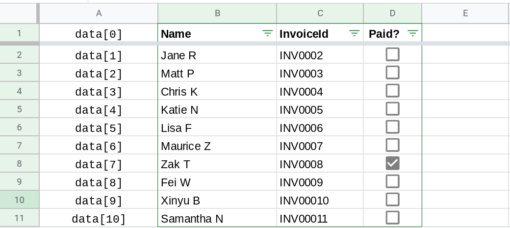
In the loop above, the variable i is set to 1 initially (usually it is set to 0 when iterating through arrays). This is because the first element in the two-dimensional array is the header row and we would never want to hide it. We use an if statement to check if the value in the 3rd column of each row is the value "Y". If it is, we hide the corresponding row. Please note that row numbers start from 1 and not 0. So, the header row is row number 1. However, the array indices start at 0. So, the first element of the array data (i.e., the header row) is at position 0 and not 1. This is why we hide the row i+1 and not i. The screenshot below shows this. The value data[0] represents row 1 and this is the header row. Therefore, if we want to hide the row corresponding to data[9], we should hide row 10.

Step 3 — Create a function to show all rows

Create a function called showAllRows() that will unhide all the rows in your sheet.

function showAllRows() {
  var sheet = SpreadsheetApp.getActive().getSheetByName("Data");
  sheet.showRows(1, sheet.getMaxRows());
}

How does the showAllRows() function work?

The function first gets a reference to the sheet named Data.

var sheet = SpreadsheetApp.getActive().getSheetByName("Data");

Then it unhides all rows using the showRows() method. The showRows() method accepts two row numbers as parameters. The rows in between these two rows will be unhidden. Since we want all the rows to be shown, we specify 1 and sheet.getMaxRows() as the two row numbers.

sheet.showRows(1, sheet.getMaxRows());

Step 4 — Create a custom menu to make it easy for users to run these functions

The final step is to create a custom menu to make it easy for you (and other users) to run the two functions. We create two menu items in the menu, one to filter rows and another to show all rows. If you're not familiar with custom menus, please refer to the tutorial on custom menus in Google Sheets.

function onOpen() {
  SpreadsheetApp.getUi().createMenu("Custom Filter")
    .addItem("Filter rows", "filterRows")
    .addItem("Show all rows", "showAllRows")
    .addToUi();
}

Full code

For your convenience, I've pasted the full code below.

//@OnlyCurrentDoc

function onOpen() {
  SpreadsheetApp.getUi().createMenu("Custom Filter")
    .addItem("Filter rows", "filterRows")
    .addItem("Show all rows", "showAllRows")
    .addToUi();
}

function filterRows() {
  var sheet = SpreadsheetApp.getActive().getSheetByName("Data");
  var data = sheet.getDataRange().getValues();
  for(var i = 1; i < data.length; i++) {
    //If column C (3rd column) is "Y" then hide the row.
    if(data[i][2] === "Y") {
      sheet.hideRows(i + 1);
    }
  }
}

function showAllRows() {
  var sheet = SpreadsheetApp.getActive().getSheetByName("Data");
  sheet.showRows(1, sheet.getMaxRows());
}

Conclusion

In this tutorial I showed you how to hide rows based on cell value in Google Sheets.

I hope you found this tutorial helpful. Thanks for reading!